Post-Quantum Discrete Gaussian Noise Samplers
The security of many modern cryptographic systems, particularly lattice-based schemes—depends on the generation of small error values sampled from discrete Gaussian distributions. In this work, we focus on designing and evaluating hardware implementations of several sampling algorithms, including Rejection Sampling, Box-Muller, and the Ziggurat method.
Our goal is to provide actionable recommendations for future adoption across cryptosystems, based on a careful analysis of sampling efficiency, hardware cost, and throughput. A key strength of our implementation is its ability to perform high-precision sampling that meets or exceeds the NIST-recommended 112-bit security level for post-quantum cryptography, an area where most existing hardware solutions fall short.
The design is highly optimized for FPGA deployment and built with generic, modular architecture, enabling seamless integration into a wide range of cryptographic systems.
Background
Noise sampling, typically from discrete Gaussian distributions—is a foundational component of lattice-based cryptography. These small error values are essential for concealing sensitive information during both key generation and encryption. Importantly, the underlying Bounded Distance Decoding (BDD) problem associated with Gaussian sampling can be reduced to the Shortest Vector Problem (SVP) or the Closest Vector Problem (CVP). These reductions form the theoretical basis for the security guarantees of lattice-based cryptographic systems.
While simpler distributions such as uniform or binomial can be used for noise sampling, they typically require significantly higher noise levels to achieve comparable security. This increase in noise introduces greater computational complexity and degrades the performance of cryptographic systems. Additionally, these distributions often suffer from information leakage and offer weaker security guarantees.
In contrast, the discrete Gaussian distribution provides a more favorable balance between security and efficiency, making it the preferred choice for many post-quantum cryptographic schemes. However, generating high-precision discrete Gaussian samples is a complex and non-trivial task. It presents a major challenge in implementing secure and performant cryptosystems, as it requires high-precision floating-point arithmeticb> to ensure minimal statistical deviation and strong security guarantees.
Ensuring resistance to side-channel attacks remains a critical challenge in the implementation of Gaussian noise samplers. Developing constant-time sampling algorithms that do not compromise performance is still an open problem. Efficient and secure implementations are difficult to achieve, as they require meticulous timing analysis to eliminate data-dependent execution paths. A robust solution must guarantee constant-time behavior while maintaining high precision, thereby minimizing the risk of information leakage and ensuring strong security guarantees in practical cryptographic systems.
Discrete Gaussian Distribution
Let E be a random variable on R, then for x ∈ R, we have
x = height of the curve’s peak
c = position of the curve’s peak
σ = standard deviation, control’s the width of the bell
σ2 = variance
Note: Smaller the width of the bell curve, narrower will be the Gaussian distribution. This has two advantages: better proof of security and small signatures in signature schemes.
1. Let E be a random variable on Z, then
2. Let E be a random variable on Z, then
The discrete Gaussian distribution DL,σ over a Lattice L with standard deviation σ > 0 assigns a probability proportional to as follows:
Let E be a random variable on L, then
Tail bound of the Discrete Gaussian distribution
Tail of the Gaussian distribution is infinitely long and cannot be covered by any sampling algorithm. We need to sample up to a bound known as the tail bound. A finite tail-bound introduces a statistical difference with the true Gaussian difference. So, the tail bound will depend on the maximum statistical distance allowed by the security parameters.
For any c > 1, the probability of sampling v from DZm,σ satisfies the following inequality
Precision Bound (Why true discrete Gaussian distribution is not feasible?)
The probabilities in a discrete Gaussian distribution have infinitely long binary representations and hence no algorithm can sample according to the true discrete Gaussian distribution. Secure applications require sampling with high precision to maintain negligible statistical distance from actual distribution.
Let ρz denote the true probability of sampling z ∈ Z according to the distribution Dz,σ
Assume that the sampler selects z with probability pz where |pz - ρz| < ε for some error constant ε > 0.
The statistical distance Δ to the true distribution DZm,σ is given by
Here,
ĎZm,σ is approximate discrete Gaussian distribution corresponding to the finite-precision probabilities pzover m independent samples.
Also,
Summary: Probability distribution function for discrete Gaussian distribution is given by
c = 0, i.e., Gaussian distribution centered around 0.
The advantage of assuming c = 0 is that there will be symmetry of probability density function and it is sufficient to generate samples over Z+ and use a random bit to determine the sign.
For practicality, generate samples in the interval [0, τσ] where τ is positive constant or tail-cut factor. Also, for practical reasons, the probabilities Dσ(x) are calculated only upto n-bit precision and can be denoted by Dnσ.
Sampling Algorithm: A sampling method is required to generate samples from discrete Gaussian distributions. Below are several sampling algorithms and their efficient hardware implementations.
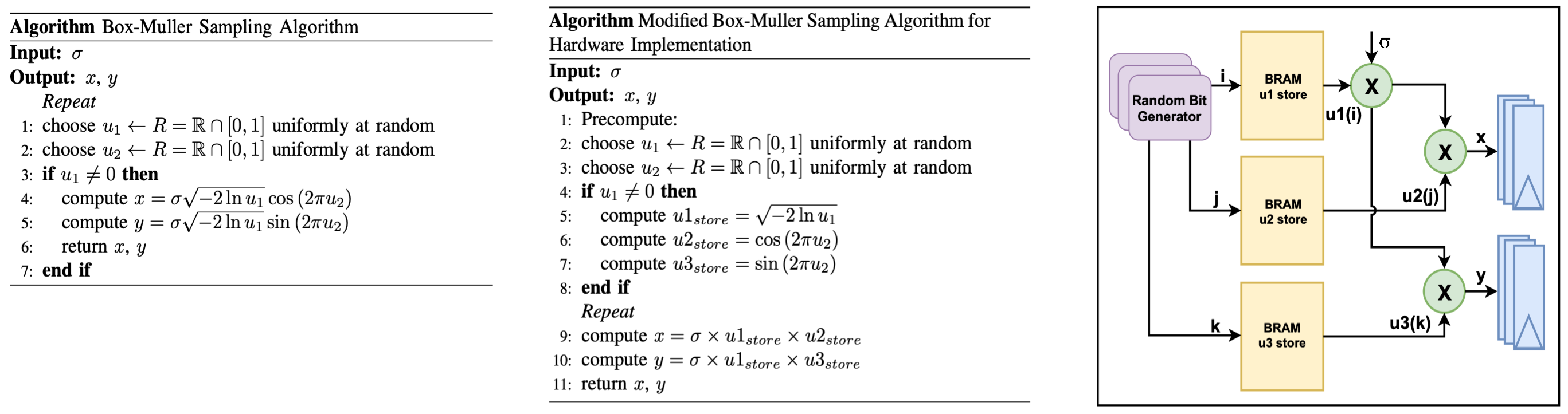
Box-Muller Sampling
The Box-Muller sampling method is derived from the Box-Muller transform, originally proposed by Box and Muller. This technique converts two uniformly distributed random values from the interval [0,1} into two samples drawn from a standard Gaussian distribution. The algorithm begins by accepting a standard deviation σ as input, which defines the target distribution. In the initial steps, two uniform random samples are generated. These are then transformed, through a series of mathematical operations into Gaussian-distributed outputs.
Each iteration of the algorithm produces two Gaussian samples, x and y, making it an efficient method for generating high-quality noise in cryptographic applications.
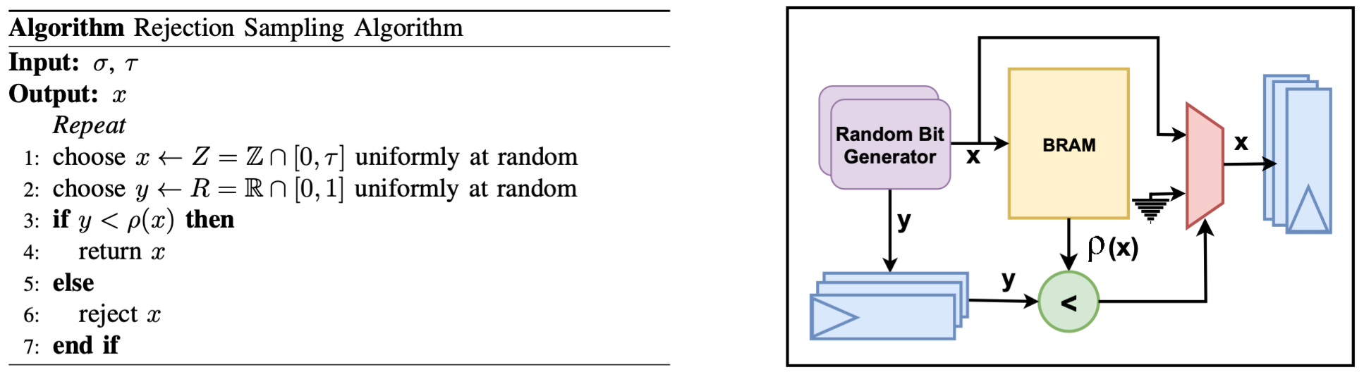
Rejection Sampling
Rejection sampling, also known as the acceptance-rejection method, is a fundamental technique for generating samples from a target probability distribution. The core idea involves uniformly sampling values from the interval [0,1] and retaining only those that fall under the curve of the desired probability density function. This method is simple and widely applicable, though its efficiency depends on the shape of the target distribution.
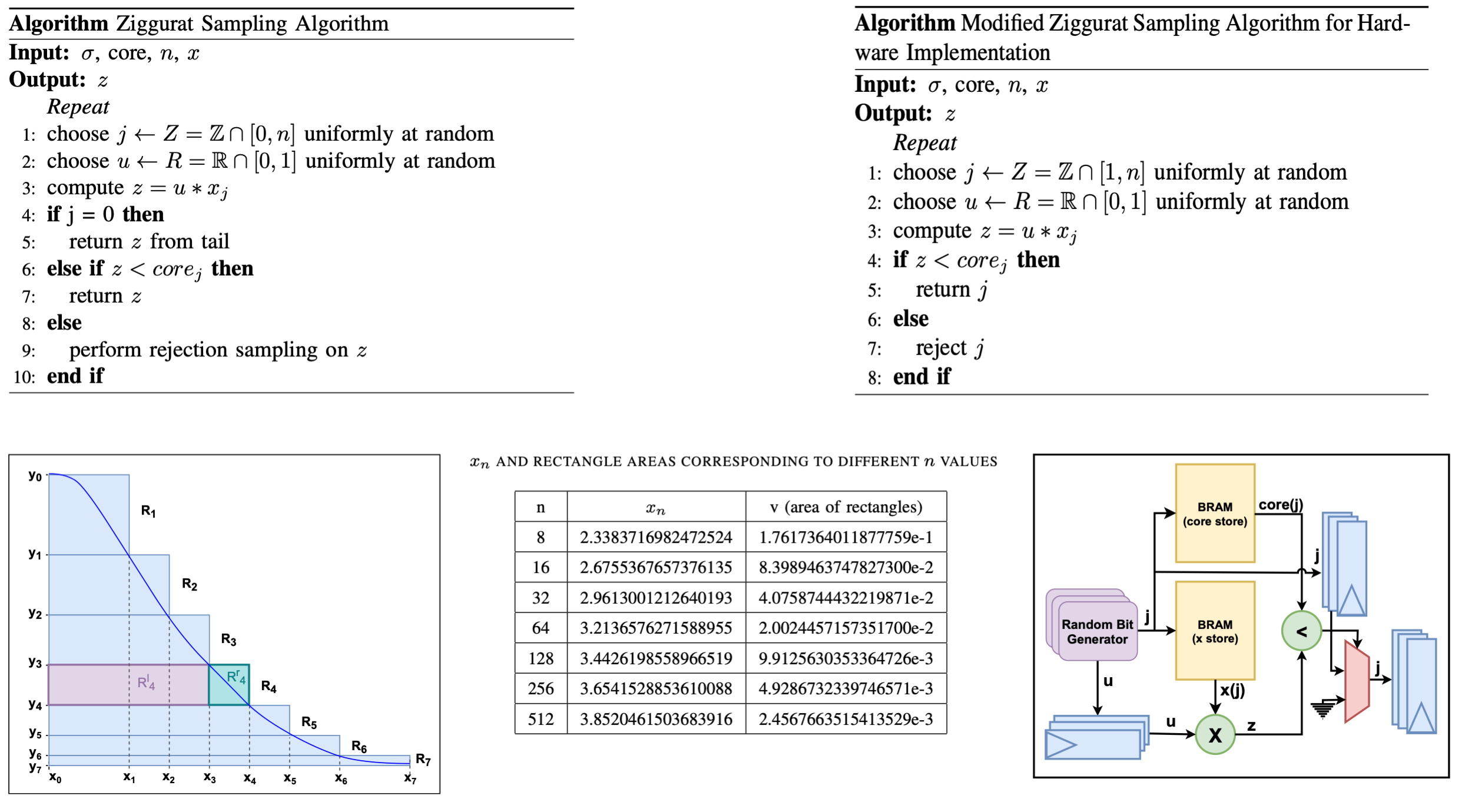
Ziggurat Sampling
Developed by Marsaglia and Tsang, the Ziggurat method is designed for sampling from monotonically decreasing probability distributions. It partitions the target distribution into horizontal, equal-area layers, resembling the stepped structure of ancient Mesopotamian ziggurats. These layers, along with a cap and tail region, form a two-dimensional step function that enables efficient sampling.
Hardware Implementation Notes
We provide highly optimized, constant-time hardware implementations of Box-Muller, Rejection, and Ziggurat sampling algorithms for Gaussian distributions. These designs are tailored for post-quantum cryptographic systems, offering:
- High-precision sampling
- Resistance to side-channel attacks
- Parameterized modules for easy integration into existing or future cryptosystems
- Performance evaluations across resource usage, sampling efficiency, and throughput offer valuable insights into selecting the most suitable sampling method for specific applications.
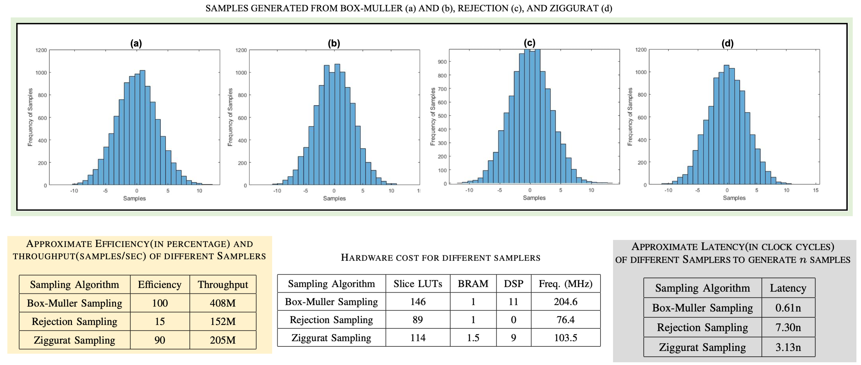
Based on our evaluations we offer the following guidance:
- Box-Muller Sampling: Highest sampling efficiency and throughput, but also the most resource-intensive. Ideal for applications where performance is critical and resource constraints are minimal.
- Rejection Sampling: Lowest resource usage, making it suitable for constrained environments or applications requiring only a small number of samples. However, efficiency and throughput may suffer when scaling.
- Ziggurat Sampling: Offers a balanced trade-off between resource utilization and sampling efficiency. Recommended for general-purpose use where both performance and resource constraints must be considered. These insights aim to support the broader research community in selecting the most appropriate Gaussian noise sampling method for their cryptographic systems.